Currently, I am working on the revision of StationRank, a paper we wrote with Vahid Moosavi. In the words of one of the academic referees: “The paper presents a Markov Chain (MC) framework to analyse daily aggregated itineraries of the swiss railway systems. They use their MC framework to asses the congestion, resilience and fragility of the railway network”. In the preprint we also discuss the relevance of a somewhat obscure notion: the Kemeny’s constant.

Preliminaries and assumptions

import math
import time
import numpy as np
from scipy import linalg as la

For this brief analysis, I assume an ergodic MC of discrete time in first order, with a row-stochastic transition probability matrix $\mathbb{P}$ . By solving $\pi^T\mathbb{P}=\pi^T$ , we obtain the stationary distribution vector $\pi^T$ and the eigenvalues $\lambda_1 = 1,\lambda_2,\dots,\lambda_n$ . Having the eigenvalues, we directly obtain the Kemeny constant $K=\displaystyle\sum_{j=2}^{n} \frac{1}{1-\lambda_j}$ ¹. This is very straightforward to calculate, but difficult to interpret. I would like to focus on another formulation in terms of mean first passage time $m_i{}_j$ which grants us more insight to the inner workings of $K$ .

Mean First Passage Time

Mean first passage time is the expected number of steps from an origin state $S_i$ to a destination state $S_j$ . The equation $K=\displaystyle\sum_{j=1}^{n} m_i{}_j \pi_j$ is yet another, more intuitive way to calculate the Kemeny constant as the average mean first passage time from any origin state to any other destination state chosen according to the probability $\pi_j$ and shows that $K$ is independent from the choice of the initial state $S_i$ .

# Calculate the Drazin inverse
I = np.identity(P.shape[0])
Q = drazin_inverse((I - P), tol=1e-4)

Obviously now, in addition to $\pi^T$ , we also need to calculate mean first passage time, which in turn requires the calculation of the group (special case of Drazin) inverse of $\Q=(\I-\mathbb{P})$ .

A matrix $\G$ is the group inverse of $\Q,$ if and only if:

$(\Q)(\G)(\Q)=(\Q)$
$(\G)(\Q)(\G)=(\G)$
$(\Q)(\G)=(\G)(\Q)$

Interpretability often comes at a cost.

def drazin_inverse(A, tol=1e-4, verbose='on'):
    """Compute the Drazin inverse of A.

    Parameters:
        A ((n,n) ndarray): An nxn matrix.

    Returns:
       ((n,n) ndarray) The Drazin inverse of A.
    """
    e1 = time.time()
    n = A.shape[0]
    f = lambda x: abs(x) > tol
    g = lambda x: abs(x) <= tol
    Q1, S, k1 = la.schur(A, sort=f)
    Q2, T, k2 = la.schur(A, sort=g)
    U = np.hstack((S[:, :k1], T[:, :n - k1]))
    U_inv = la.inv(U)
    V = U_inv @ A @ U
    Z = np.zeros((n, n))
    if k1 != 0:
        Z[:k1, :k1] = la.inv(V[:k1, :k1])        
    return U @ Z @ U_inv

The mean first passage time can be calculated as follows: $\m_i{}_j = \frac{g_j{}_j - g_i{}_j}{\pi_j}$ .

# Calculate Mean First Passage Time
MFPT = np.zeros(shape=(n, n))
for i, row in (enumerate(G)):
    for j, _ in enumerate(row):
        if j != i:
	    m = (G[j][j] - G[i][j]) / pi[j]
	    MFPT[i][j] = m

Takeaway

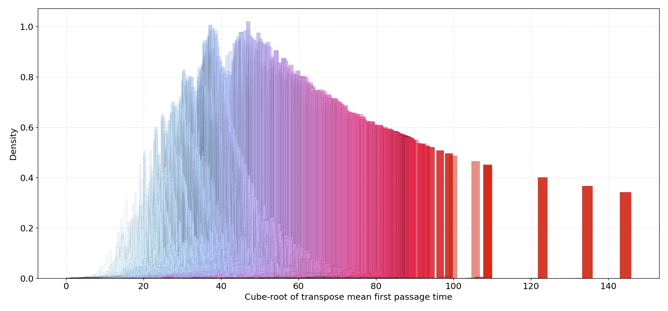
If instead of $\m_i{}_j$ , which by definition is expected to have very similar distribution for different initial stations, we have a look at the mean $\m_j{}_i$ , then we come up with a kind of accessibility analysis in terms of “remoteness” of train stations. This can be easily verified on a map. 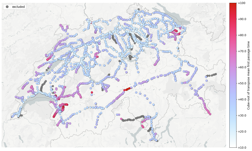hist remote Geographic distribution of mean $m_j{}_i$ , a measure of “remoteness”

1: E. Crisostomi, S. Kirkland & R. Shorten (2011) A Google-like model of road network dynamics and its application to regulation and control, International Journal of Control, 84:3, 633-651, DOI: 10.1080/00207179.2011.568005