Emerging technologies such as Unmanned Areal Vehicles (UAV), commonly referred to as drones, effectively change the way we see the world. Their disruptive potential propagates across multiple areas of human activity and most certainly in science and engineering. Unprecedented amounts of valuable data streams are being collected constantly in high resolution and at relatively low cost. There are different ways to think about the implications of such technologies, but I would like to argue here that they present a certain chance to democratize knowledge. Evidence being collected by these ubiquitous mobile sensors also invites us to rethink scientific practice and challenge established theories.

Recently, a team of researchers from the Laboratory of Urban Traffic Systems (LUTS) of the EPFL introduced a new era of traffic monitoring with the pNEUMA experiment [1]. A swarm of drones flew over the busy center of Athens recording at high frequency the precise position, velocity and acceleration of multiple types of vehicles. The resulting dataset is freely available online for academic use. While similar datasets exist for freeways, pNEUMA monitors urban traffic phenomena. For this demonstration, I used data collected from a major arterial between 9:30 and 10:00 on a weekday during heavy congestion.

Outline of the methodology

This work has some methodological similarities with [5] as it approaches the study of traffic stream characteristics from a signal-processing standpoint. This idea is very appealing because it is well posed for spatiotemporal data mining and discovery of hidden patterns in massive and noisy data. However, the physical interpretation of such signals is of equal, if not higher, importance and neither the authors of [5], nor those of [4], provide convincing answers in this regard. Further, an important prerequisite for this analysis is map-matching of the raw trajectories to the underlying urban street network [12]. Since the matching is part of preprocessing, a detailed discussion is well beyond the scope of my post. Interested readers are encouraged to study the classic paper [8] and the code implementation [9]. Last but not least, a notebook accompanying my analysis is also open source and publicly available on Github.

matcher = DistanceMatcher(map_con,
                          max_dist=300,
                          min_prob_norm=0.0001,
                          obs_noise=20,
                          max_lattice_width=8,
                          avoid_goingback=True,
                          non_emitting_states=False)
states, _ = matcher.match(route)

Parade of algorithms: PCA, SOM, DBSCAN and lane assignment

The next hard problem after map-matching is lane assignment and it can be solved in three steps:

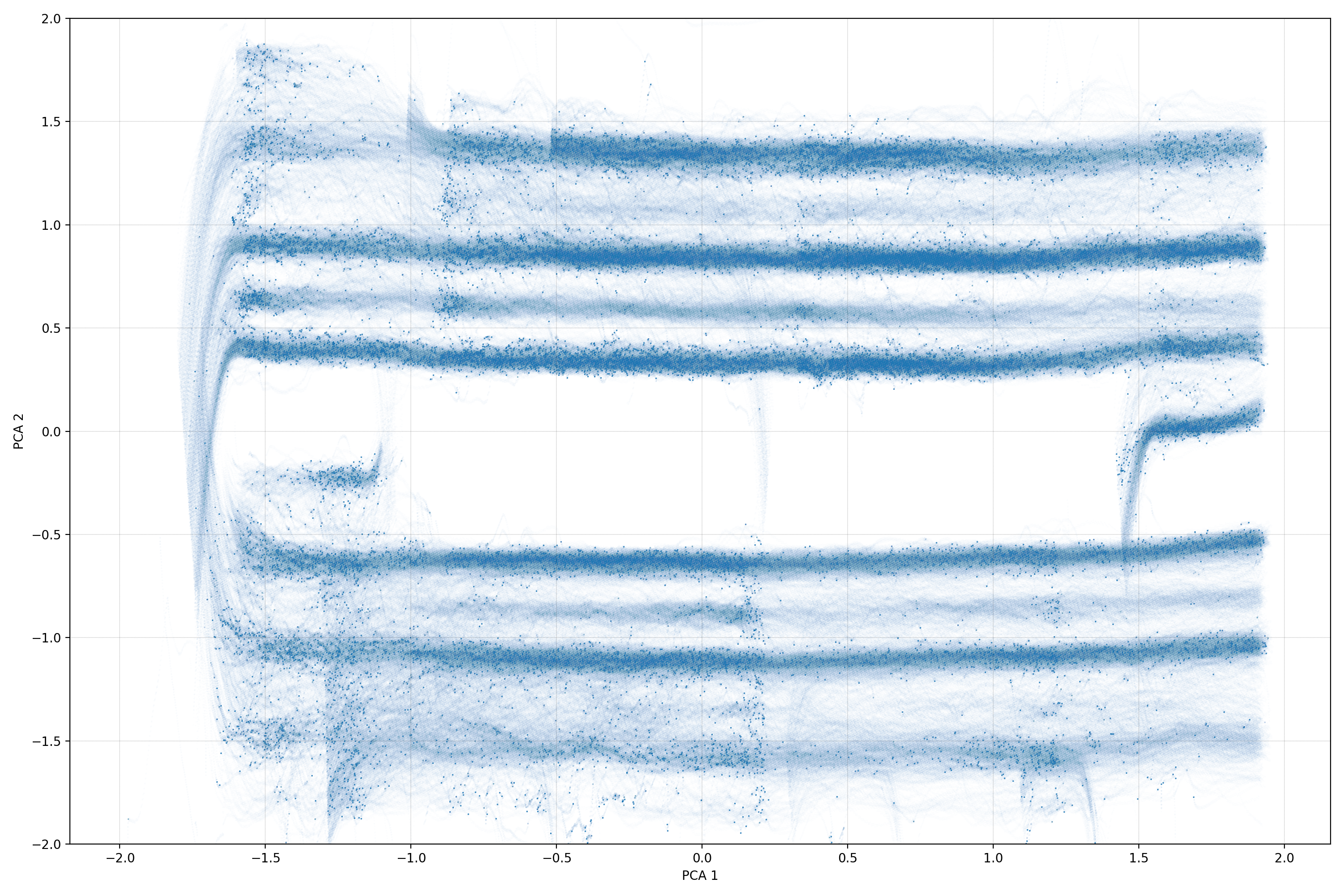
Principle component analysis (PCA) [13]. This efficient algorithm detects the orthogonal directions which maximize variance. Combined with a standard scaler, it maps tuples of latitude and longitude on a rotated system of zero mean and unit variance. Interestingly enough, apart from the three main lanes of the arterial, an additional lane of motorcycles emerges on the fast side of both streams.
Data reduction with self organizing maps (SOM) [14]. Now, given that we are looking at traces of 3000 vehicles over 20 minutes with a framerate of 25 fps, clustering becomes a big-data challenge. Self organizing maps reduce the complexity of the task by means of unsupervised pre-indexing. SOM assigns the original points to groups of topology preserving best matching units (bmus).
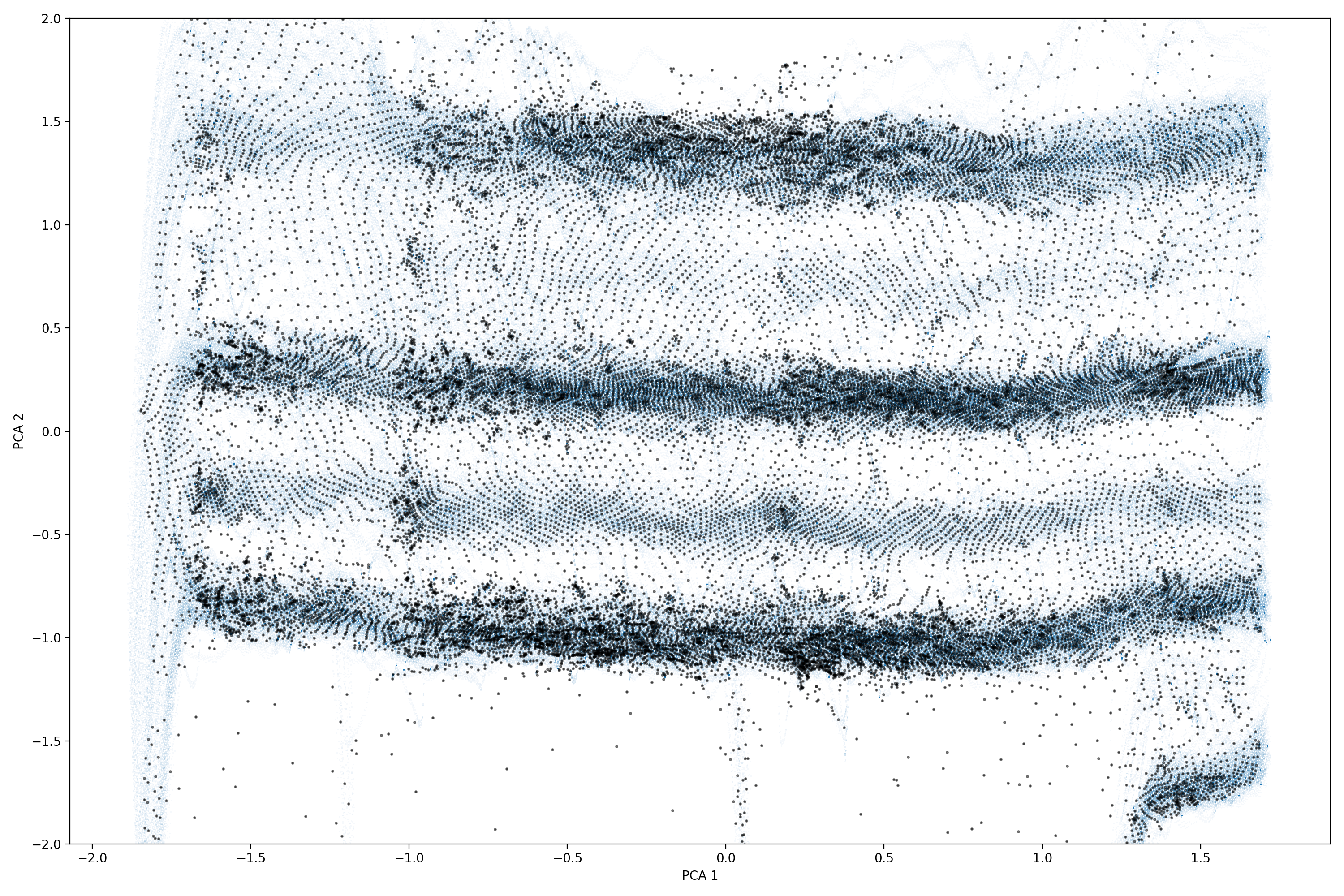
Density-based spatial clustering (DBSCAN) [13]. This algorithm does a good job on the reduced dataset of bmus. It successfully identifies not only the primary lanes, but also the emergent one.

Why is lane assignment so crucial in the first place? A simple answer is that the problem can become significantly easier if we reduce the notion of space to one dimension of distance traveled. This means that lane-changing vehicle trajectories have to be split and assigned to the respective lane. Now the 2D plane can be used for spatiotemporal studies, which are known as time-space diagrams. The following figure shows the inbound traffic lanes of Alexandras avenue from leftmost to rightmost under extreme congestion with characteristic stop and go wave patterns. It is worth mentioning that the emergent lane of powered two wheelers operates under a totally different regime close to free flow.

The problem of spatiotemporal binning

One way to obtain traffic quantities of interest, is to divide the space-time grid into bins of size $\Delta X \times \Delta T$ in which we can safely assume that velocity, density and flow remain constant [5] [4]. For a total length $L$ and observation interval $T$ , a bin is given by the following expression: ${\mathrm{Bin}}_{i,j} = \left[ {i{ \Delta }X,\left( {i \+ 1} \right){ \Delta }X} \right] \times \left[ {j{ \Delta }T,\left( {j \+ 1} \right){ \Delta }T} \right]_{i \in \left( {0 \ldots n_{\mathrm{x}}} \right),j \in \left( {0 \ldots n_{\mathrm{t}}} \right)}$ , where $n_x = \frac{L}{ \Delta X }$ and $n_t = \frac{T}{ \Delta T }$ . Each ${\mathrm{Bin}}_{i,j}$ might contain a non empty set of traces ${\mathrm{trace}}_{i,j} = \{ \mathrm{trace} | \mathrm{trace} \in {\mathrm{Bin}}_{i,j} \}$ with a velocity vector $\mathbf{V}_{\mathrm{trace}}_{i,j}.$ The collective speed of the bin is simply $\hat V_{i,j} = \mathrm{Mean}\left( \mathbf{V}_\mathrm{trace}_{i,j} \right)$ . An approximation for density is given by merely counting the number of traces in the bin (the cardinality of the set $\mathrm{trace}_{i,j}$ ), normalized by the cell size and the sampling rate: $\hat \rho_{i,j} = \frac{\mathrm{Card}(\mathrm{trace}_{i,j})}{ \Delta X \Delta T \mathrm{Sampling} \,\, \mathrm{Rate}}$ . Flow is then obtained as $\hat Q_{i,j} = \hat V_{i,j}\hat \rho _{i,j}$ .
Binning can be implemented quite elegantly in scientific python:

from scipy import stats
for i, lane in enumerate(lanes):
    x = list(lane.time)
    y = list(lane.distances)
    u = list(lane.speed)
    count = stats.binned_statistic_2d(x, y, None, 'count', bins=[binx, biny])
    density = (count[0].T) / (dx * dy * rate * 1000)
    speed = stats.binned_statistic_2d(x, y, u, 'mean', bins=[binx, biny])
    speed = speed[0].T
    NaNs = np.isnan(speed)
    speed[NaNs] = 0
    flow = density * speed

Unfortunately, this simple approach has major theoretical limitations, as it is not immediately obvious what is the optimal bin size. In [4], we see that any attempt to use central limit theorem reasoning is a bad idea since independence of variables is violated (traces of the same vehicle). They propose a double histogram optimization for traces and vehicles with the objective of securing a robust estimate. While it is clear that better binning helps, it will always introduce frequencies that are external to our data thus distorting the original continuous flow. A second approach is to refrain from binning altogether by employing the concept of virtual loop detectors [3]. To my understanding, detectors bring their own meta-parameters together with the additional question of their optimal placement and population.

NMF recovery of traffic density

Let us pause for a moment and speculate the existence of a methodological alternative. If the binning treatment introduces some arbitrary, physically meaningless frequency to the data, then it should be quite easy to mask that frequency and keep only useful signals. For the sake of argument, I will just reuse binning settings from [5], namely $\Delta X = 6m$ and $\Delta T = 5s$ . Obviously a sub-optimal choice because the density histograms of the freeway and those of the arterial most probably differ. The binned spatiotemporal matrix $\mathbf{M}$ is then decomposed such as $\mathbf{M} \approx \mathbf{W} \mathbf{H}$ [10]. This is called non-negative matrix factorization (NMF), a matrix decomposition with a strict constraint of non-negativity. NMF has a very broad scope of applications and it comes in many flavors [2]. The idea here is quite simple: find the most faithful lower rank representation of the spatial and temporal signals that is free of noise!

The figure below shows the binned version of the density matrix for all lanes, side by side with their corresponding NMF reconstructions. While the two matrices still have exactly the same shape, or number of pixels, the one appears “blocky” and the the other “natural” with a much more continuous color spectrum. It can be shown that this method is surprisingly independent of the bin size given the appropriate level of dimensionality (number of components).

model = NMF(n_components=n_components,
        init='random',
        random_state=10,
        max_iter=500)
W = model.fit_transform(all_metrics[i][0])
H = model.components_
reconstructed = np.inner(W, H.T)

If the authors of [5] or [4] had drawn the fundamental diagram of traffic flow [7], they would have observed something similar to the first row of the following panel, or at best, its optimized version. There are very strong, suspiciously regular artefacts. The density spike for example at $166.6 veh/km$ equals exactly $1000/6$ . Same is true for the horizontal lines at $720veh/h$ which is equal to $3600/5$ and so on. This distortion can be safely attributed to the particular bin dimensions of $6m$ and $5s$ respectively. Another alarming indication is the relatively high concentration of points with zero density and speed.

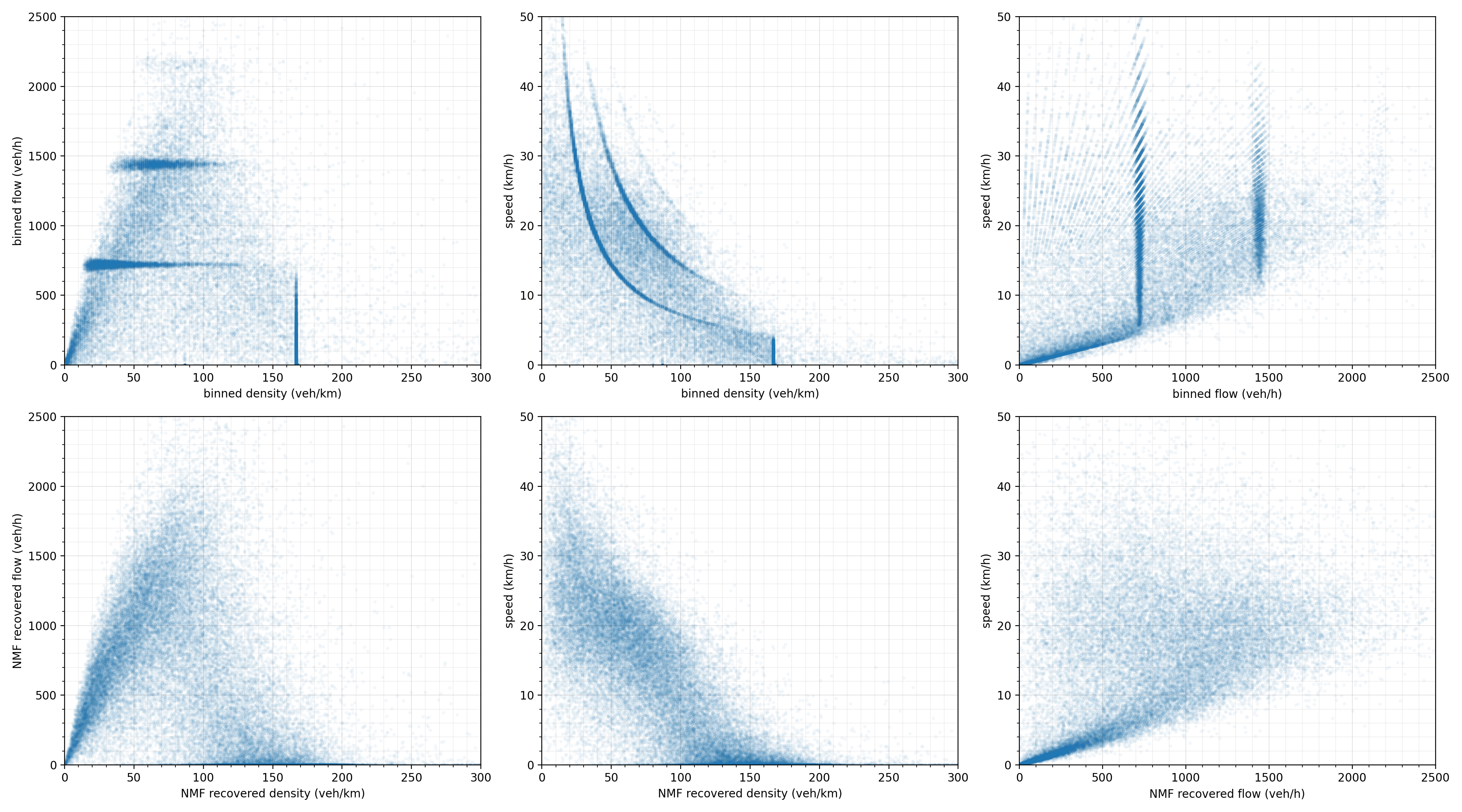
Clearly, NMF is able to cancel out the binning frequencies by keeping only physically interpretable spatial and temporal signatures. The shape of the resulting plots is in agreement with current theory [6]. Furthermore, we see for example that the binned jam density was displaced by more than twenty points. It is also worth mentioning that each plot shows all lanes drawn on top of each other.

The fundamental diagram lives in 3D

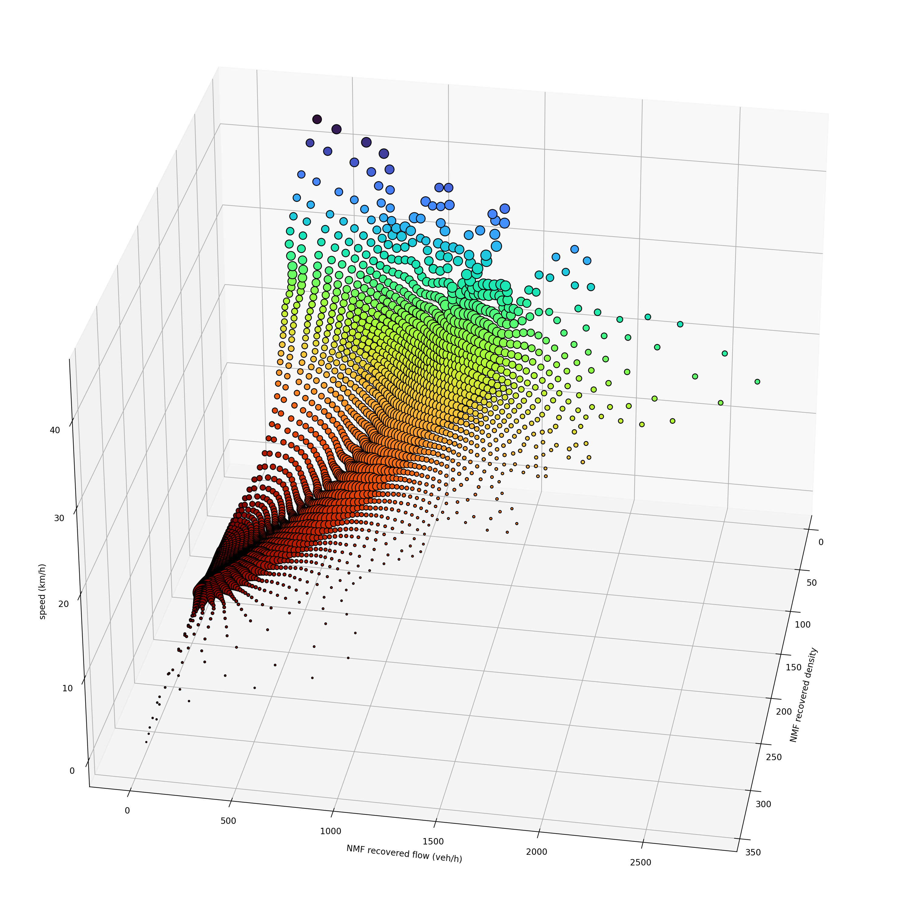
If it is still unclear how the three variables relate to each other, we can plot them in 3D. By virtue of the fundamental equation $\hat V_{i,j} = \frac{\hat Q_{i,j}}{ \hat \rho _{i,j}}$ , all points lie on a surface of the form $z = \frac {x} {y}$ . This is known from the 70’s as “the surface of admissible traffic stream models” [7]. But what is much more interesting, is the particular distribution of the points that constitutes a model. The final figure shows a SOM fit of the 3D fundamental diagram for the studied arterial stream with color representing velocity. The overall shape is now easier to comprehend as a triangular cut of the 3D surface with distinct free flowing, congested and jammed regimes. The three diagrams above simply show projections of a continuous object.

3dfd

Conclusion

Robust data-driven reconstructions of the fundamental diagram are beneficial for two main reasons. Existing microsimulation tools that are in need of validation can benefit from accurate representations of field data. Finally, on the aggregate level, a better understanding of the traffic dynamics at individual links directly affects the study of macroscopic, networkwide phenomena.

Aknowledgement

Data source: pNEUMA – open-traffic.epfl.ch

References

[1] Emmanouil Barmpounakis, Nikolas Geroliminis, On the new era of urban traffic monitoring with massive drone data: The pNEUMA large-scale field experiment, Transportation Research Part C: Emerging Technologies, Volume 111, 2020, Pages 50-71, ISSN 0968-090X, https://doi.org/10.1016/j.trc.2019.11.023.

[2] Mohammadreza Saeedmanesh, Nikolas Geroliminis, Clustering of heterogeneous networks with directional flows based on “Snake” similarities, Transportation Research Part B: Methodological, Volume 91, 2016, Pages 250-269, ISSN 0191-2615, https://doi.org/10.1016/j.trb.2016.05.008.

[3] Thomas Courbon, Ludovic Leclercq, Cross-comparison of Macroscopic Fundamental Diagram Estimation Methods, Procedia - Social and Behavioral Sciences, Volume 20, 2011, Pages 417-426, ISSN 1877-0428, https://doi.org/10.1016/j.sbspro.2011.08.048.

[4] Francois Belletti, Mandy Huo, Xavier Litrico, Alexandre M. Bayen, Prediction of traffic convective instability with spectral analysis of the Aw–Rascle–Zhang model, Physics Letters A, Volume 379, Issue 38, 2015, Pages 2319-2330, ISSN 0375-9601, https://doi.org/10.1016/j.physleta.2015.05.019.

[5] Avila, A.M., Mezić, I. Data-driven analysis and forecasting of highway traffic dynamics. Nat Commun 11, 2090 (2020). https://doi.org/10.1038/s41467-020-15582-5

[6] van Wageningen-Kessels, F., van Lint, H., Vuik, K. et al. Genealogy of traffic flow models. EURO J Transp Logist 4, 445–473 (2015). https://doi.org/10.1007/s13676-014-0045-5

[7] Gerlough, Daniel L., and Matthew J. Huber. Traffic Flow Theory: A Monograph. Transportation Research Board, National Research Council, 1975.

[8] Paul Newson and John Krumm. 2009. Hidden Markov map matching through noise and sparseness. In Proceedings of the 17th ACM SIGSPATIAL International Conference on Advances in Geographic Information Systems (GIS ‘09). Association for Computing Machinery, New York, NY, USA, 336–343. DOI:https://doi.org/10.1145/1653771.1653818

[9] Meert, Wannes, and Verbeke, Mathias. HMM with Non-Emitting States for Map Matching. 2018.

[10] Lee, D., Seung, H. Learning the parts of objects by non-negative matrix factorization. Nature 401, 788–791 (1999). https://doi.org/10.1038/44565

[11] Graser, Anita. “MovingPandas: Efficient Structures for Movement Data in Python.” GI_Forum, vol. 1, 2019, pp. 54–68. DOI:https://doi.org/10.1553/giscience2019_01_s54

[12] Boeing, G. 2017. OSMnx: New Methods for Acquiring, Constructing, Analyzing, and Visualizing Complex Street Networks. Computers, Environment and Urban Systems 65, 126-139. DOI:https://doi.org/10.1016/j.compenvurbsys.2017.05.004

[13] Scikit-learn: Machine Learning in Python, Pedregosa et al., JMLR 12, pp. 2825-2830, 2011.

[14] SOMPY: A Python Library for Self Organizing Map (SOM) V Moosavi, S Packmann, I Vallés https://github.com/sevamoo/SOMPY.

Useful links with analysis of the same dataset: