Most football fans (please don’t call it soccer), are not fond of penalties and I readily agree with them. We cannot accept that randomness alone basically determines the outcome of the game. But, when it comes down to solving engineering problems, penalties are essential. Therefore, I would like to share with you what I have learned about penalties in the context of vehicle trajectory reconstruction.

Source: Unsplash

In the last post, I presented some preliminary work on the pNEUMA dataset, a collection of naturalistic vehicle trajectories captured by a swarm of drones hovering over the dense urban fabric of Athens city. This massive dataset along with suggested applications was introduced in [1]. In fact, the research potential of this new kind of empirical evidence, motivated me to start my PhD at EPFL LUTS and work directly with the authors, Prof. Geroliminis and Dr. Barmpounakis.

Of course vehicle trajectory datasets collected in the wild, even with state of the art methods, are noisy. Many researchers in the field of intelligent transport systems (ITS) have attempted to recover or reconstruct noise-free vehicle trajectories, such as [3], [4] and [7]. Simply speaking, there exist two kinds of noise: white noise and anomalies. White noise is assumed to be independently and identically distributed with constant variance and zero mean.

The above assumptions do not apply to anomalies that can be described as assymetric, abrupt events. Anomalies are also different from outliers, extreme but feasible values of an underlying phenomenon. Outliers are valuable and should be preserved along the process. Some authors, such as [7], do not draw this distinction and refer to all undesirable values as outliers.

Just use the Butterworth filter

In theory, anomaly detection should not be that complicated, especially if you ask someone with background in applied math. And so I did just that. The answer was: “just use the Butterworth filter”. More formally, the magnitude squared frequency response of an $N$ th order Butterworth filter with cut-off frequency $\Omega_{c}$ is given by

$|H ( \Omega )|^{2} = \frac{1}{1 \+ \epsilon^{2}({\Omega}/{\Omega_{c}} )^{2 N}}$ [11].

If $\epsilon=1$ , there is a gain of approximately $-3$ dB at the critical frequency $\Omega_{c}$ . A very nice property of this filter is having “maximally flat magnitude” in the pass band [6]. In contrast to simple moving averages, which tend to oscillate in the low frequencies, the Butterworth filter suppresses only high frequencies.

Surprisingly, in spite the excellent denoising properties of this filter, in the literature of vehicle trajectory reconstruction it is not used for anomaly detection, but rather as a smoothing technique, see [4] and [7]. More specifically, [7] impose predetermined thresholds on longitudinal acceleration according to some not very convincing argumentation and [4] detect anomalies with a more involved rule-based system.

Here I will demonstrate how a single Butterworth filter specification with $N=2$ and $\Omega_{c}=0.9$ Hz can be used for detecting anomalies in two trajectory metrics: speed $v$ and azimuth $\theta$ . As you might suspect, there is a catch: we are not primarily interested in the filtered metrics $\widetilde{v}, \widetilde{\theta}$ as such, but rather in the absolute differences $|v-\widetilde{v}|, |\theta-\widetilde{\theta}|$ . For ease of notation and regardless of the metric considered, we will refer to such absolute differences as some error function $y$ , which is specific to each vehicle.

from scipy.signal import butter, freqz, filtfilt
fs = 25 # Sampling frequency
fc = .9 # Cut-off frequency
wc = fc / (fs / 2)
N = 2 # Filter order
b, a = butter(N, wc, 'low')
speed_signal = df.speed
speed_filter = filtfilt(b, a, speed_signal)
azimuth_signal = df.azimuth
azimuth_filter = filtfilt(b, a, azimuth_signal)

At its current form, $y$ cannot be used for anomaly detection. Now the problem is that, strictly speaking, $y$ is not even a function, but rather a set of (noisy) observations $y_j$ at $n$ consecutive timestamps $t_j$ . Therefore, our objective is to find a nice analytical expression for $y$ in continuous time, which is smooth.

Functional data analysis helps

The motivation of having a smooth error function comes from the assumption that neighboring anomalous observations should be strongly and positively autocorrelated. To reiterate, anomalies are not anything like white noise: they are “non-stationary, autocorrelated errors” [9]. Fitting non-stationary error functions can be lots of fun (no pun intended). Fortunately, there is a whole branch in statistics called functional data analysis (FDA) [5], [9], [10], [12], [13], that provides us with the mathematical machinery required for such problems.

To start with, we assume an error model $y_j=x(t_j)\+\epsilon_j$ , where $x(t_j)$ is a continuous, smooth analytical expression evaluated at time $t_j$ and $\epsilon_j$ is some residual term. Our objective is to find that function $x(t)$ , such that the residuals are minimized and the function is as smooth as possible. In other words, we have regularized functional regression. We further assume that this model is additive and $x(t)$ is constructed from a linear combination of $K$ simpler basis functions $\phi_k(t)$ , such that $x(t_j)=\sum_{k}^{K}c_k\phi_k(t_j)$ . We point the reader to [5] for details on these functions. Then we can specify a least squares estimation problem

$\text{SSE}(\mathbf{c}) = \sum_{j}^{n} [y_{j} - \sum_{k}^{K}c_k\phi_k(t_j)]^{2} = \sum_{j}^{n} [y_{j} - \mathbf{\phi}^{'}(t_{j})\mathbf{c} ]^{2}$ ,

where $\mathbf{c}$ is the vector of coefficients ${c_k}$ and $\mathbf{\phi}^{'}(t_{j})$ is the ${j}$ th row of the ${n}$ by ${K}$ matrix $\mathbf{\Phi}$ with $\mathbf{\Phi}_j{}_k=\phi_k(t_j)$ . Next, we measure the roughness of the function $x(t)$ by introducing our long-awaited penalty term, the “integrated squared second derivative or total curvature” [10]

$\text{PEN}_2(x) = \int [D^{2}x(t)]^{2} d t$ ,

where the bounds of integration coincide with the start and end time of each trajectory (omitted here). Then, we can formulate the final expression to be minimized as

$\text{PENSSE}_\lambda(\mathbf{c}) = \text{SSE}(\mathbf{c})\+\lambda\text{PEN}_2(x)$ [9], [10], [12], [13],

where the smoothing hyperparameter $\lambda$ is chosen by the “generalized cross-validation criterion” [10]

$\text{GCV} \left(\lambda\right) = \left(\frac{n}{n - df (\lambda)}\right) \left(\frac{\text{SSE}}{n - df (\lambda)}\right)$ .

The degree of freedom of the fit $df (\lambda)$ can be found if we define a “symmetric roughness penalty matrix” $R = \int \mathbf{\phi}(t) \mathbf{\phi}^{'}(t) d t$ of order $K$ and let $df (\lambda) = \text{trace} \left[\mathbf{\Phi}(\mathbf{\Phi}^{'} \mathbf{\Phi} \+ \lambda\mathbf{ R})^{- 1} \mathbf{\Phi}^{'}\right]$ [10].

The number of basis functions used is proportional to the duration of each trajectory, as in [12] and [13].

from pygam import LinearGAM, s
n_basis = int(np.round(max(t) - min(t))) + 2
speed_error = abs(speed_filter - speed_signal)
y = speed_error
gam = LinearGAM(s(0, n_splines=n_basis)).gridsearch(t, y, progress=False)
df['speed_error'] = gam.predict(t)
azimuth_error = abs(azimuth_filter - azimuth_signal)
y = azimuth_error
gam = LinearGAM(s(0, n_splines=n_basis)).gridsearch(t, y, progress=False)
df['azimuth_error'] = gam.predict(t)

Seeking the (ground) truth

So far, we obtained error functions per trajectory for speed and azimuth. Clearly, we also need to specify the respective thresholds of what is considered anomalous. Please note that thresholds are set on the error functions $y_v, y_\theta$ and not directly on the metrics of interest $v, \theta$ . Let us assume for now that such thresholds $y_t$ are known. If $y>y_t$ , the respective observations of interest are marked as anomalous and are removed from the dataset. The missing values are then interpolated linearly. Finally, we obtain anomaly-free speed $v^{*}$ and azimuth $\theta^{*}$ .

It is known that the majority of authors validate their reconstructions based on longitudinal acceleration. Here, we will break away from this tradition and propose an alternative method based on speed and lateral acceleration. More importantly, we will show that our approach also puts constraints on longitudinal acceleration, although indirectly. Therefore, we calculate the noise free longitudinal acceleration $a_{lon}^{*}=dv^{*}/dt$ and lateral acceleration $a_{lat}^{*}={v^{*}}^{2}d\theta^{*}/ds^{*}$ , where $s^{*}=\int v^{*} d t$ .

In absence of any ground truth, we will use insights gained from a study with instrumented vehicles [2]. The authors make some very interesting and strong arguments based on the theory of human-machine interaction and attempt to deduce its governing laws. They propose a “modified Levinson criterion” [2] that sets the feasible bounds on lateral acceleration as a function of speed. This “Bosetti criterion” is

${a_{lat}^{Bosetti}}=\frac{a_0}{\sqrt{(1-{(v^{*}/{v}_0)}^2)^2\+ 2{(v^{*}/{v}_0)}^2 }}$ , with ${a_0}=5.22 m/{s^2}, v_0 = 14.84 m/s = 53.42 km/h$ .

Every observation that is found outside of the feasible domain, as described by the Bosetti equation, is considered anomalous. This basically sets an upper bound for our reconstruction. Now we just need to specify the lower bound. Notice how close we are to the feasible domain without even using smoothing.

More penalties

In principle, the anomaly-free distribution, as described in the previous section, can shrink arbitrarily in absence of a regularization mechanism that penalizes false positives. To this end, we introduce a beautiful in its simplicity heuristic: a calibration point is chosen such that the expected anomaly count in its immediate vicinity is close to zero. Both speed and azimuth anomalies are included in the count.

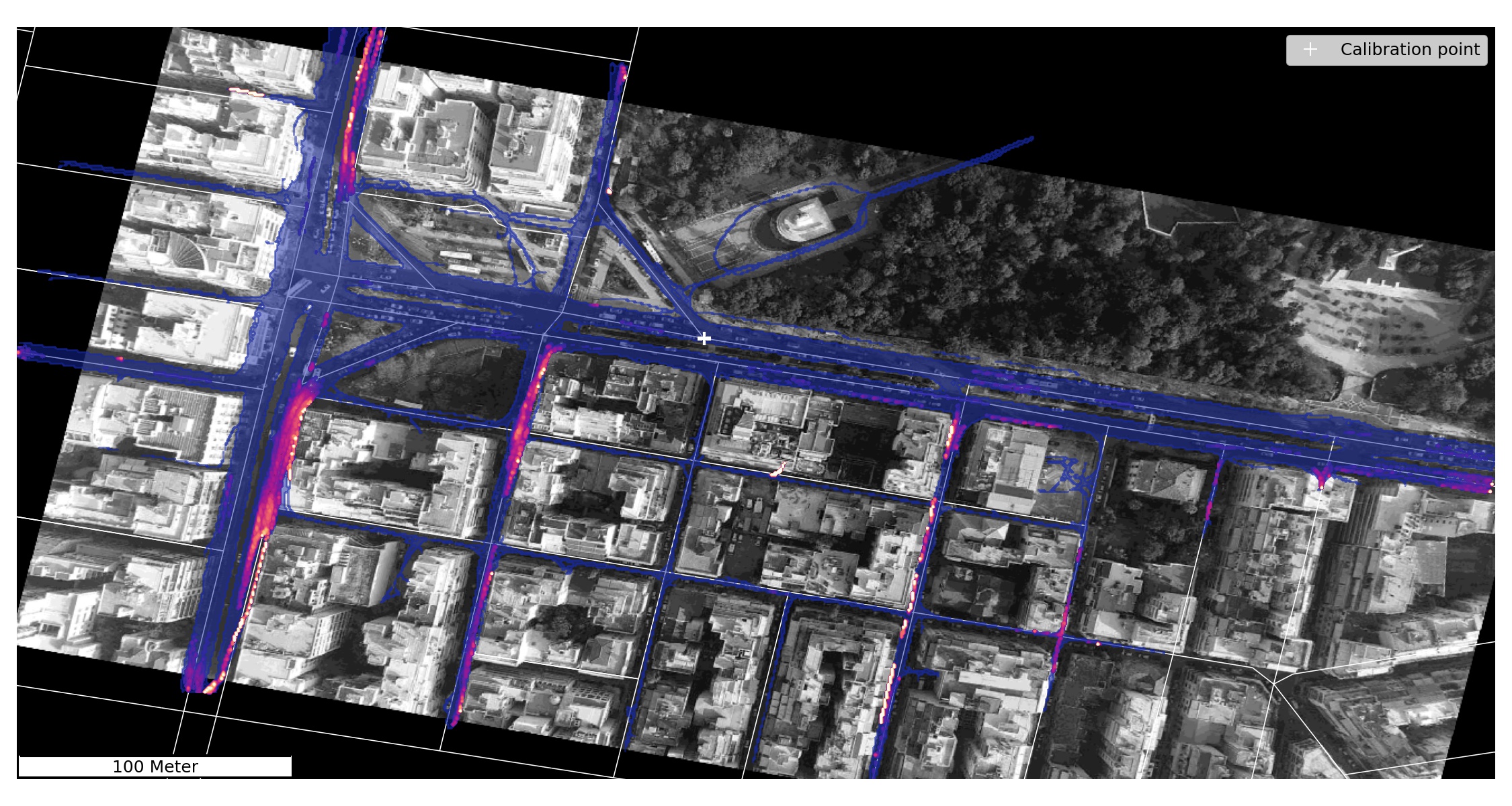Speed anomaly heatmap 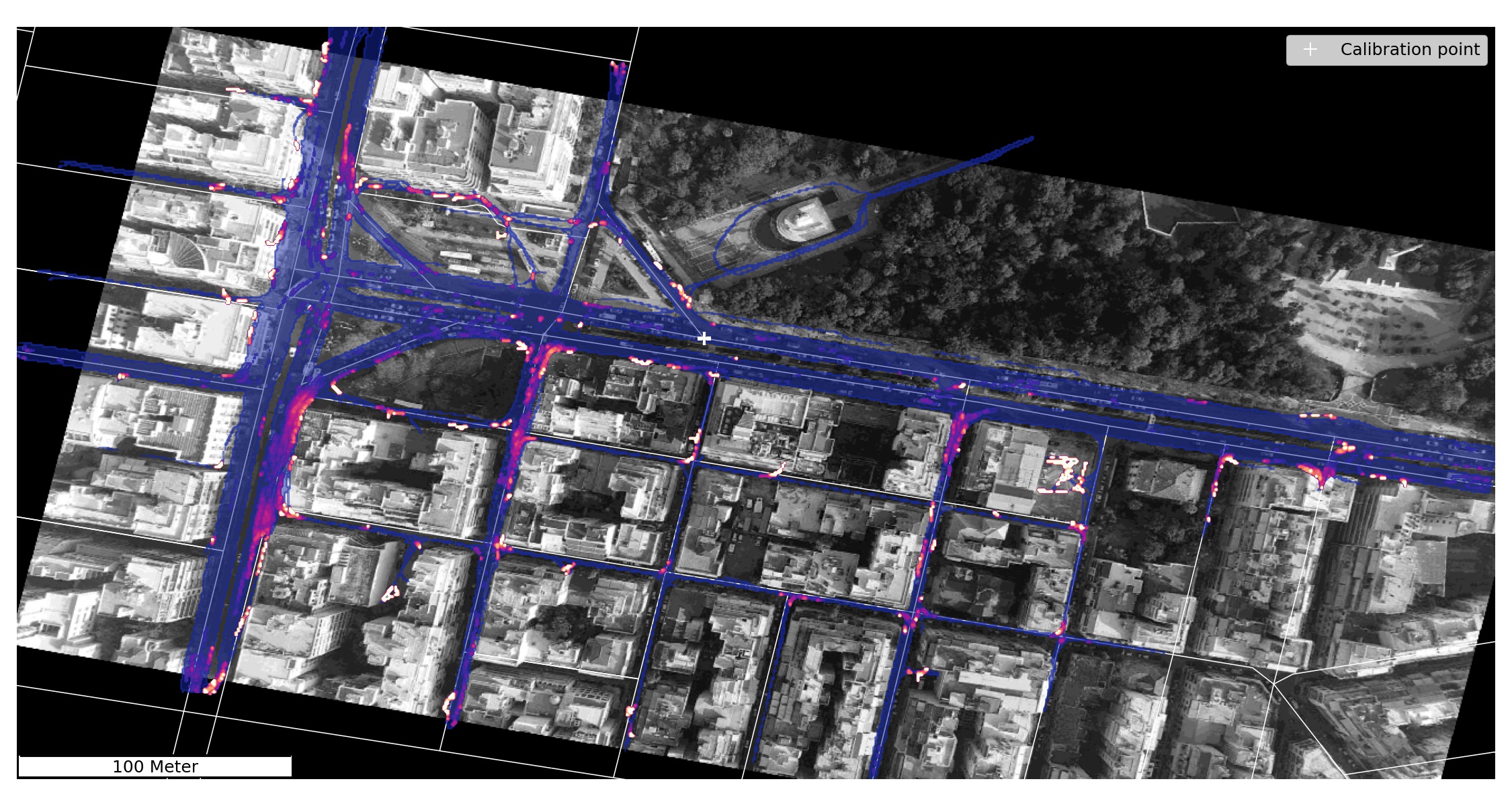Azimuth anomaly heatmap

The calibration point is placed there where no visual restrictions or perspective distortions are expected. We set the vicinity radius $r = 3m$ . The heatmap of speed anomalies shows that the main arterial has virtually no anomalous observations. Both figures support our hypothesis of spatial autocorrelation.

The loss function wins

By now we have gained a qualitative understanding of the objective and we proceed to formulate a two-dimensional optimization problem by minimizing the following loss function

$\L({y_t^v, y_t^\theta})=\sum_{m}^{M}\{|a_{lat}(m)|-a_{lat}^{Bosetti}(m)\}\+\mathrm{Card}\{p|\mathrm{d}(p,q)<r\}$ ,

where $\y_t^v, y_t^\theta$ are the speed and azimuth error thresholds, $M$ is the total number of undetected anomalous observations (false negatives) and the last term is the cardinality of the set of misclassified points $p$ that fall within a distance $r$ from the calibration point $q$ (false positives). It turns out that this unusual loss function has a single, well defined global optimum (minimum) and it is convex. Please be aware that this statement holds true for the chosen filter specification with $\Omega_{c}=0.9$ Hz. Higher cut-off frequencies perform poorly and lower cut-off frequencies produce multiple minima.

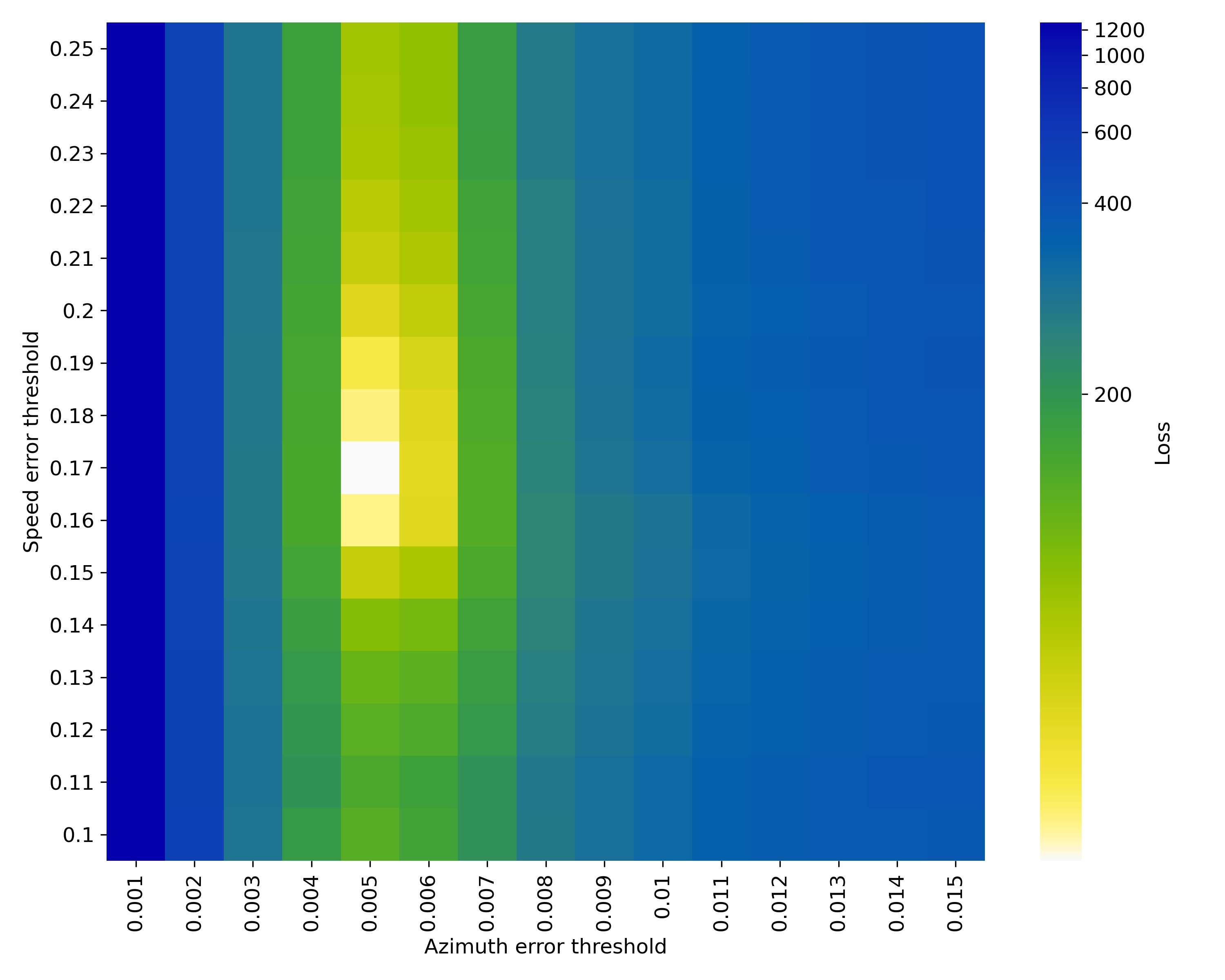
The optimization is done by multi-threaded, direct evaluation on a $15\times15$ grid and the search ranges have been identified by inspection. Notice that the two thresholds differ by one order of magnitude. Inside the optimum grid cell, polishing in the form of local search finds the exact threshold parameters.

With the optimal parameters in place, we can quantify the errors in the dataset. These are summarized in the following table. We distinguish between contamination rates and anomaly rates. A trajectory is contaminated if any of its observations is anomalous. Static points are excluded in anomaly counts.

Anomaly statistics	speed	azimuth	both	union
Portion of contaminated vehicle trajectories.	19.62%	25.61%	11.85%	33.39%
Portion of anomalous data, excluding staypoints.	0.81%	0.93%	0.24%	1.5%

The final touch

As mentioned in the beginning, we make a clear distinction between anomalies and white-noise. Previous research has focused too much on the second type of errors with extensive use of smoothing. This is not necessarily due to poor judgment, but can be also attributed to the very poor quality of existing datasets [3]. In reality, most of the contribution to the noise comes from the first type of errors. Nevertheless, if we want smooth accelerations, white-noise should be also treated.

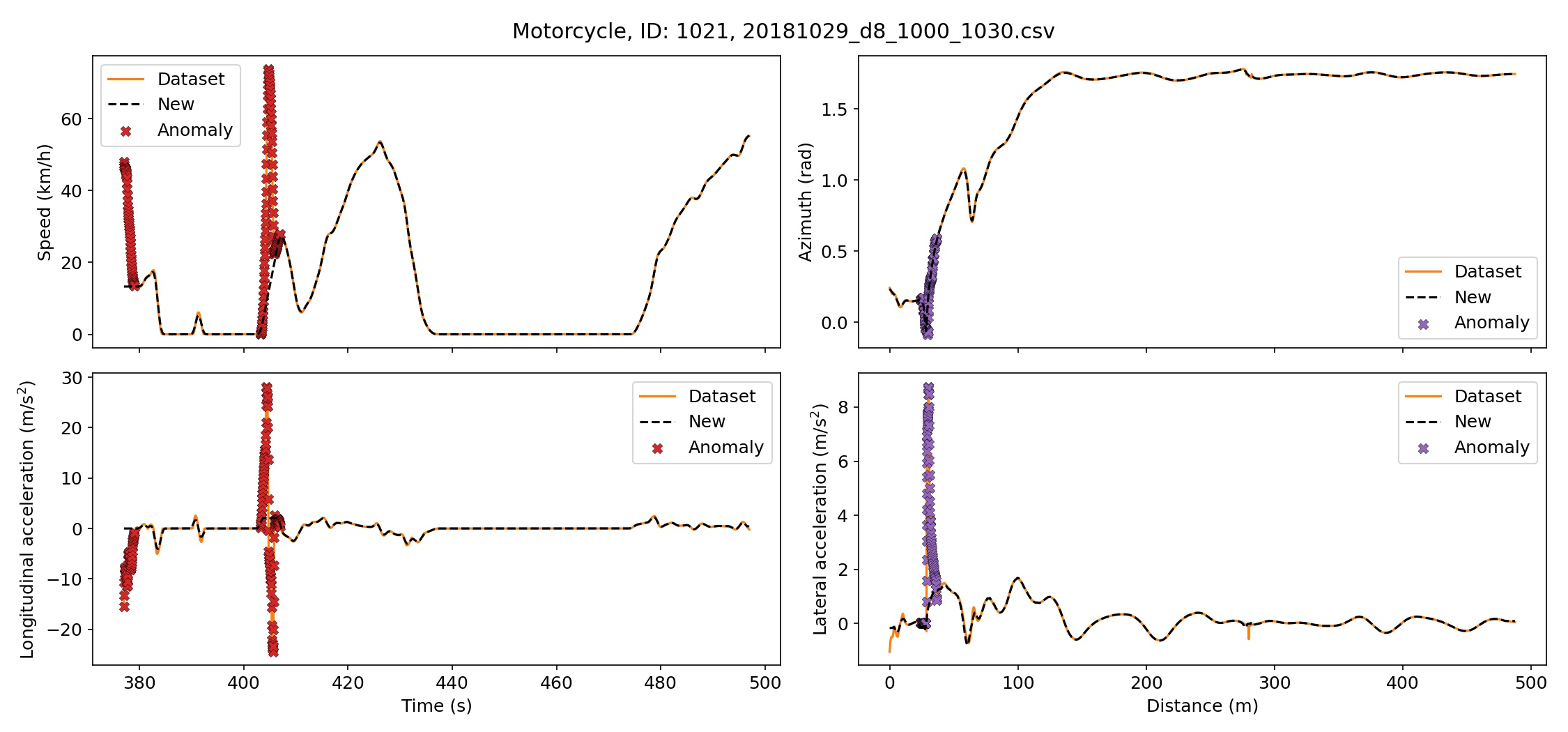
For the elimination of white-noise, we use a first order Savitzky-Golay filter with a window length equal to the frame rate (25 fps). This is equivalent to a centralized moving average. Centralized moving averages are a good choice for offline data as they do not introduce delay effects [6]. The SG filter is applied on the anomaly-free data. From the level of a single vehicle trajectory to the distribution of accelerations in the dataset, before and after reconstruction, we can see how our treatment reduces the noise without introducing noticeable systematic oversmoothing.

Before closing, I reiterate that the above distributions exclude static points, known also as staypoints. This is very important and it has been recently shown [8] that static and moving vehicles are completely different phenomena and should be treated separately. Attention to this fact has been drawn only after the emergence of detailed data on urban traffic.

On another note, some authors put emphasis on the importance of internal and external consistency of vehicle trajectory reconstructions [7]. This idea is interesting, but not without significant shortcomings, see [3] for a detailed criticism. We should add here, that especially the concept of external, or platoon consistency fails to account for the spatial autocorrelation of the errors among neighboring trajectories.

In summary, we presented a novel detection method for speed and for azimuth anomalies. We managed to recover, as faithfully as possible, the underlying distributions of longitudinal and lateral accelerations for six different modes of transport without hand-crafted rules. Our method can be used for quantifying autocorrelated errors or, inversely, for identifying network segments that are devoid of errors and can thus be used directly for validation of traffic flow models or for traffic safety analytics.

Acknowledgement

Data source: pNEUMA – open-traffic.epfl.ch.

Special thanks goes to Dr. Gustav Nilsson for his elaboration on the Butterworth filter. His suggestions have been crucial to my work. It is surprising how much one can learn during a coffee break.

References

[1] Barmpounakis, Emmanouil, and Nikolas Geroliminis. “On the New Era of Urban Traffic Monitoring with Massive Drone Data: The PNEUMA Large-Scale Field Experiment.” Transportation Research. Part C, Emerging Technologies, vol. 111, 2020, pp. 50–71, doi:10.1016/j.trc.2019.11.023.

[2] Bosetti, Paolo, et al. “On the Human Control of Vehicles: An Experimental Study of Acceleration.” European Transport Research Review, vol. 6, no. 2, 2014, pp. 157–170, doi:10.1007/s12544-013-0120-2.

[3] Coifman, Benjamin, and Lizhe Li. “A Critical Evaluation of the Next Generation Simulation (NGSIM) Vehicle Trajectory Dataset.” Transportation Research Part B: Methodological, vol. 105, 2017, pp. 362–377, doi:10.1016/j.trb.2017.09.018.

[4] Dong, Shuoxuan et al. “An Integrated Empirical Mode Decomposition and Butterworth Filter Based Vehicle Trajectory Reconstruction Method.” Physica A 583.126295 (2021): 126295. doi:10.1016/j.physa.2021.126295.

[5] Eilers, Paul H. C., and Brian D. Marx. “Flexible Smoothing with B-Splines and Penalties.” Statistical Science: A Review Journal of the Institute of Mathematical Statistics, vol. 11, no. 2, 1996, pp. 89–121, doi:10.1214/ss/1038425655.

[6] Haslwanter, Thomas. Hands-on Signal Analysis with Python: An Introduction. Springer International Publishing, 2021.

[7] Montanino, Marcello, and Vincenzo Punzo. “Trajectory Data Reconstruction and Simulation-Based Validation against Macroscopic Traffic Patterns.” Transportation Research Part B: Methodological, vol. 80, 2015, pp. 82–106, doi:10.1016/j.trb.2015.06.010.

[8] Paipuri, Mahendra, et al. “Empirical Observations of Multi-Modal Network-Level Models: Insights from the PNEUMA Experiment.” Transportation Research. Part C, Emerging Technologies, vol. 131, no. 103300, 2021, p. 103300, doi:10.1016/j.trc.2021.103300.

[9] Ramsay, J. O., and B. W. Silverman. Functional Data Analysis. Springer New York, 2005.

[10] Ramsay, James, et al. Functional Data Analysis with R and MATLAB. Springer New York, 2009.

[11] Taylor, Fred. Digital Filters : Principles and Applications with MATLAB. 1st ed., Wiley-IEEE Press ;IEEE Xplore, 2011.

[12] Yang, Di, et al. “A Functional Approach for Characterizing Safety Risk of Signalized Intersections at the Movement Level: An Exploratory Analysis.” Accident; Analysis and Prevention, vol. 163, no. 106446, 2021, p. 106446, doi:10.1016/j.aap.2021.106446.

[13] Yang, Di, et al. “Proactive Safety Monitoring: A Functional Approach to Detect Safety-Related Anomalies Using Unmanned Aerial Vehicle Video Data.” Transportation Research. Part C, Emerging Technologies, vol. 127, no. 103130, 2021, p. 103130, doi:10.1016/j.trc.2021.103130.